04. Sorting and Searching

ADM Sorting Searching

Fundamental Searching and Sorting Algorithms

Algorithm	Time Complexity	Best Use Case
Heapsort	O(n log n)	Priority queues and large datasets
Mergesort	O(n log n)	Stable sorting for linked lists
Quicksort	O(n log n) avg.	General-purpose fast sorting
Insertion Sort	O(n²)	Small datasets
Binary Search	O(log n)	Searching sorted arrays

Applications of Sorting

Sorting provides a foundation for many other algorithms, facilitating the following applications:

• Binary Search : data needs to be sorted in order to achieve O(log n) time complexity
• Closest Pair Search : sorted lists allow scanning for closest elements in O(n) time
• Duplicate Detection : checking adjacent elements in a sorted list helps find duplicates efficiently
• Frequency Distribution : Counting of occurrences is straightforward in a sorted list
• Selection Problem : extracting the k-th element
• Geometric Algorithms : finding convex hulls in computational geometry

Pragmatics of Sorting

• Quadratic Algorithms O(n²) : Work well for small datasets (e.g. insertion sort, bubble sort)
• Efficient Algorithms (O n log n) : Necessary for large datasets (e.g. quicksort, merge sort)
• Stability in Sorting : A stable sort maintains the relative order of equal elements (e.g. merge sort)
• In-Place Sorting : Algorithms like heapsort sort data within the original array, minimizing space complexity

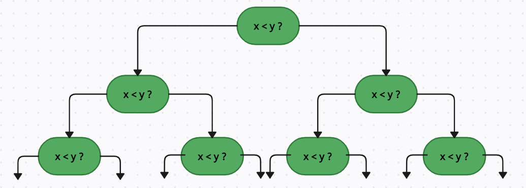
Theoretical Limit for Comparison Based Sorting

• in algorithm design, O(n log n) is often the best possible time complexity we can achieve
• this is because in the worst case there are n! possible orderings for n elements
• Decision Tree Model : sorting can be represented as a binary decision tree
  • since comparison splits the outcomes, the tree height (and number of comparisons) must be at least O(n log n)

Sorting Algorithms

1. Heapsort

Heap Sort

• Time Complexity: O(n log n)
• In-Place: Uses a binary heap data structure.
• Application: Suitable for large datasets where memory efficiency is important.

Steps:

1. Build a max-heap.
2. Extract the maximum element and place it at the end.
3. Heapify the remaining elements.

---

2. Mergesort

Merge Sort

• Time Complexity: O(n log n)
• Stable Sorting: Maintains the relative order of equal elements.
• Not In-Place: Requires extra space for merging.

Steps:

1. Divide the list into two halves.
2. Recursively sort both halves.
3. Merge the sorted halves.

---

3. Quicksort

Quick Sort

• Time Complexity:
  • Average: O(n log n)
  • Worst-case: O(n²)
• In-Place Sorting: Uses partitioning.
• Randomized Version: Reduces the chance of hitting the worst case.

Steps:

1. Choose a pivot element.
2. Partition the array around the pivot.
3. Recursively sort the partitions.

---

4. Insertion Sort

Insertion Sort

• Time Complexity: O(n²)
• Efficient for Small Arrays: Performs well with nearly sorted data.
• In-Place Sorting: Requires no extra space.

Steps:

1. Start from the second element.
2. Compare it with previous elements and place it in the correct position.

---

Binary Search Algorithm

Binary Search

• Time Complexity: O(log n)
• Application: Works only on sorted arrays.

Steps:

1. Compare the target with the middle element.
2. If equal, return the index.
3. If smaller, search the left half; if larger, search the right half.

Hashing in Searching

Hashing Hash functions play a crucial role in quick look-ups

• Chaining : stores collisions in linked-lists, ensuring efficiency even with many collisions
• Open Addressing : Resolves collisions by probing the next available slot in the hash table

Take-Home Lessons

• Sorting is often the first step toward solving complex problems
• Efficient algorithms general employ O(n log n) sorting methods
• Hashing complements searching by enabling constant-time-look-ups